Stata: Graphing Distributions

Graphing Distributions

This post will demonstrate how:

1. Use the `twoway function’ plotting command to visualize distributions
2. Add colored shading to a graph to visualize portions of a distribution

The twoway function command

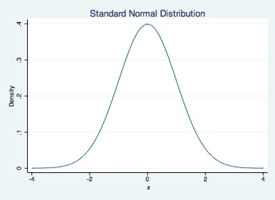
The twoway function plotting command is used to plot functions, such as y = mx + b. If we want to plot the density of a normal distribution across a range of x values, we type y=normalden(x). You can also include graphing options available to twoway plots (e.g., xtitle).

twoway function y=normalden(x), range(-4 4) xtitle("{it: x}") ///
ytitle("Density") title("Standard Normal Distribution")

Add Shading to a Figure

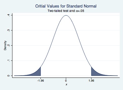
Suppose we want to shade parts of a distribution above (or below) a particular critical value. For example, we can shade a normal distribution above 1.96 and below -1.96 if we want critical values for a two-tailed test with an alpha-level of .05. To do this we will draw 3 graphs.

1. A normal curve from -4 to -1.96
2. A normal curve from -1.96 to 1.96
3. A normal curve from 1.96 to 4

The choice of -4 and 4 as upper and lower bounds is arbitrary. You can connect the three graphs by using a double pipe, ||, between calls to the twoway function command. We will shade the area under the curve for #1 and #3 using the recast(area) option of twoway function. We will assign the color of the shading to dark navy blue using the color(dknavy) option. We will leave the area under the curve for #2 unshaded.

twoway function y=normalden(x), range(-1.96 1.96) color(dknavy) || ///
function y=normalden(x), range(-4 -1.96) recast(area) color(dknavy) || ///
function y=normalden(x), range(1.96 4) recast(area) color(dknavy) ///
xtitle("{it: x}") ///
ytitle("Density") title("Critial Values for Standard Normal") ///
subtitle("Two-tailed test and {&alpha}=.05") ///
legend(off) xlabel(-1.96 0 1.96)

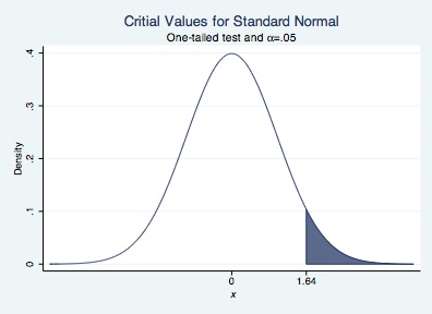
We can repeat for a one-tailed test.

twoway function y=normalden(x), range(-4 1.64) color(dknavy) || ///
function y=normalden(x), range(1.64 4) recast(area) color(dknavy) ///
xtitle("{it: x}") ///
ytitle("Density") title("Critial Values for Standard Normal") ///
subtitle("One-tailed test and {&alpha}=.05") ///
legend(off) xlabel(0 1.64)

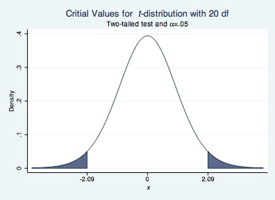
We can also visualize other distributions available in Stata. Below, I provide an example of a t-distribution with 20 degrees of freedom

twoway function y=tden(20,x), range(-2.09 2.09) color(dknavy) || ///
function y=tden(20,x), range(-4 -2.09) recast(area) color(dknavy) || ///
function y=tden(20,x), range(2.09 4) recast(area) color(dknavy) ///
xtitle("{it: x}") ///
ytitle("Density") title("Critial Values for {it: t}-distribution with 20 df") ///
subtitle("Two-tailed test and {&alpha}=.05") ///
legend(off) xlabel(-2.09 0 2.09)