Predicted Scores and Residuals in Stata
01 Oct 2013Predicted Scores in Stata
As we discussed in class, the predicted value of the outcome variable can be created using the regression model. For example, we can use the auto dataset from Stata to look at the relationship between miles per gallon and weight across various cars. We estimate the follow equation
sysuse auto
regress mpg weight
      Source |       SS       df       MS              Number of obs =      74
-------------+------------------------------           F(  1,    72) =  134.62
       Model |   1591.9902     1   1591.9902           Prob > F      =  0.0000
    Residual |  851.469256    72  11.8259619           R-squared     =  0.6515
-------------+------------------------------           Adj R-squared =  0.6467
       Total |  2443.45946    73  33.4720474           Root MSE      =  3.4389
------------------------------------------------------------------------------
         mpg |      Coef.   Std. Err.      t    P>|t|     [95% Conf. Interval]
-------------+----------------------------------------------------------------
      weight |  -.0060087   .0005179   -11.60   0.000    -.0070411   -.0049763
       _cons |   39.44028   1.614003    24.44   0.000     36.22283    42.65774
------------------------------------------------------------------------------
Thus, we see a negative relationship between weight and mpg. For every 1 unit increase in weight, mpg goes down by -.006. We can obtain the predicted scores for the observations in our dataset with the following command:
predict mpg_pred
This creates a new variable called mpg_pred with the predicted mpg for all the weight values in our dataset. Here’s 20 of the actual mpg values and 20 of the predicted values.
list mpg mpg_pred in 1/20
     +----------------+
     | mpg   mpg_pred |
     |----------------|
  1. |  22   21.83483 |
  2. |  17   19.31118 |
  3. |  22   23.57735 |
  4. |  20   19.91205 |
  5. |  15   14.92484 |
     |----------------|
  6. |  18    17.3884 |
  7. |  26   26.04091 |
  8. |  20   19.73179 |
  9. |  16   16.12658 |
 10. |  19   19.01075 |
     |----------------|
 11. |  14   13.42267 |
 12. |  14    16.0064 |
 13. |  21   13.66302 |
 14. |  29   26.76196 |
 15. |  16   17.26823 |
     |----------------|
 16. |  22   20.33266 |
 17. |  22   20.09231 |
 18. |  24    22.9164 |
 19. |  19   18.83049 |
 20. |  30   26.70187 |
     +----------------+
Residuals in Stata
Recall the a residual in regression is defined as the difference between the actual value of and the predicted value of (or ):
Thus, to compute residuals we can just subtract mpg_pred from mpg. Stata will do this for us using the predict command:
predict mpg_res, residuals
Here’s 20 of the actual mpg values, 20 of the predicted values, and 20 of the residuals.
 list mpg mpg_pred mpg_res in 1/20
     +----------------------------+
     | mpg   mpg_pred     mpg_res |
     |----------------------------|
  1. |  22   21.83483    .1651688 |
  2. |  17   19.31118   -2.311183 |
  3. |  22   23.57735    -1.57735 |
  4. |  20   19.91205    .0879486 |
  5. |  15   14.92484    .0751587 |
     |----------------------------|
  6. |  18    17.3884    .6115971 |
  7. |  26   26.04091   -.0409119 |
  8. |  20   19.73179    .2682092 |
  9. |  16   16.12658   -.1265787 |
 10. |  19   19.01075   -.0107484 |
     |----------------------------|
 11. |  14   13.42267    .5773304 |
 12. |  14    16.0064   -2.006405 |
 13. |  21   13.66302    7.336983 |
 14. |  29   26.76196    2.238046 |
 15. |  16   17.26823   -1.268229 |
     |----------------------------|
 16. |  22   20.33266    1.667341 |
 17. |  22   20.09231    1.907688 |
 18. |  24    22.9164    1.083605 |
 19. |  19   18.83049    .1695122 |
 20. |  30   26.70187    3.298132 |
     +----------------------------+
We can see that the residuals are intact the difference between the first two columns.
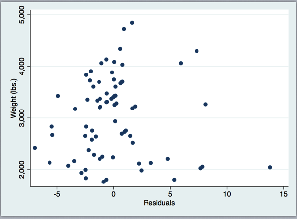
Given that the residuals are the part of the mpg that is unrelated to weight, mpg_res should be uncorrelated with weight. Let’s check:
. corr weight mpg_res
(obs=74)
             |   weight  mpg_res
-------------+------------------
      weight |   1.0000
     mpg_res |   0.0000   1.0000

Magic!