Stata: Dummy Coding

Introduction

This post will illustrate how to:

1. Use the generate and replace commands to create dummy variables.
2. A second use of the generate command to dummy variables that is simpler that #1.
3. Using tabluate to create dummy variables.

Dummy coding is used when you have nominal categories, meaning the groups are assigned a value for coding purposes, but the values don’t represent more or less of anything. For example, I might code three different categories of race and coded them as follows: Caucasian = 1, African American = 2, Hispanic = 3. The numbers are for coding purposes only, 3 is not actually any bigger or more than 1. But if we use these in a regression (or any other) analysis, the numbers will be treated as continuous - not categorical. So we need to create dummy variables. Generally, we create k-1 new groups, where k is the total number of groups, and one group is used as the reference sample, or the group we want to compare other groups to.

Method 1: Using generate and replace

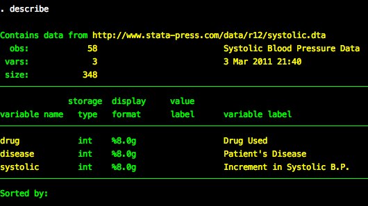
We’ll use the built in system data systolic.

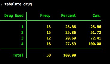
The drug variable has 4 levels.

Consequently, we’ll need to make 3 dummy coded indicator variables to represent drug. We’ll use level 4 as the reference category. We’ll use a series of generate and replace commands to create the variables. This is definitely the brute-force way to make the variables, but it makes the logic behind creating dummy variables clear.

generate drug1=1 if drug==1
replace drug1=0 if drug!=1
generate drug2=1 if drug==2
replace drug2=0 if drug!=2
generate drug3=1 if drug==3
replace drug3=0 if drug!=3

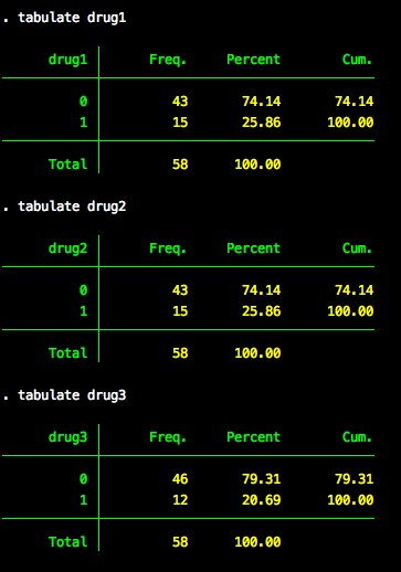
Tabulating each of the dummy variables – drug1 - drug3 – we see they match our original tabulation.

Method 2: Use generate only

We can also use a feature of the generate command to create a new variable that takes on the values 1 and 0. So, for example, if we want to create drug1, where drug1 is equal to 1 when the drug condition equals 1, we say:

generate drug1=drug==1

This creates a variable that is 1 when drug equals 1 (recall that == is a logical evaluator) and 0 any other time. If we want to use the fourth condition as the reference category, we repeat the generate command for drug2 and drug3.

generate drug2=drug==2
generate drug3=drug==3

Method 3: Use the generate option of tabulate

The function tabulate has an option called generate. The generate option takes one argument called stubname, where stubname is the stub of the new variable names created by the option. In our examples so far, the stub has been drug. Unlike the examples we have done so far, this method will create as many dummy variables as there are levels of the categorical variable (4 in our case). In our example, we type:

tabulate drug, generate(drug)

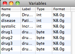
We now have four new variables in our dataset – drug1-drug4.

Stata: Labeling & Recoding Data

Labeling Variables

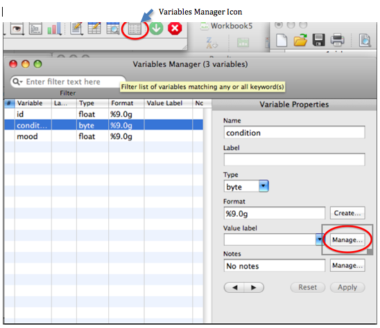
In order to assign labels to values of your variable, you can use either the variables manager or command syntax. For example, if you wanted to assign labels to each condition, where 1 represents No treatment, 2 represents Treatment A, 3 represents Treatment B & 4 represents Treatment C, you could double-click on the variable manager & click on “condition” and then “Manage.”

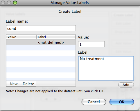
When the Manage Value Label box appears, click “Create Labels” and it will open a new dialogue box where you can give a label name to the variable and then assign labels for particular values. After you assign all of your values, be sure to click “Apply” back in your Variables Manager window.

To create labels using commands, you would use the label command. The syntax is:

label define labelname value "name"
label define cond 1 "No tx" 2 "Tx A" 3 "Tx B" 4 "Tx C"

To apply your labels, use the label command again. The syntax is label value variable labelname

label value condition cond

Recoding Data

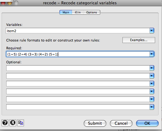
You will often need to recode values in your data for a number of reasons. For example, you may need to reverse-score items negatively-worded items on a measure. To do this via point and click, Go to Data -> Create or Change Data -> Other Variable Transformation Commands -> Recode Categorical Variable. In the Main tab, you will enter the variable(s) you want recoded and in the “Required” window, you will enter how you want them recoded. This is an example of how you might reverse score a 5-pt Likert item.

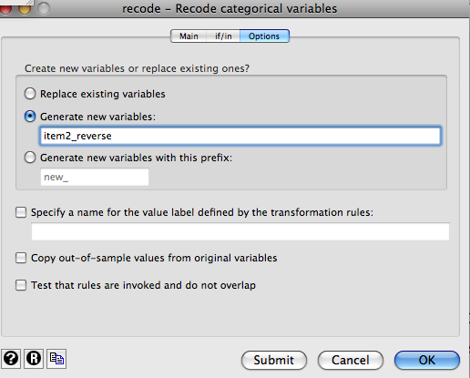
If you’re done, click “Ok”. If you want to retain your original variable and create a new variable for the reverse-scored item, go to the “Options” tab and enter the name of the new variable(s).

It is also quick and easy to recode variables using the recode command:\

recode item2 (1=5) (2=4) (3=3) (4=2) (5=1)

If you wanted to create a new variable with the recoded values, just use the clonevar command first, which will create a new variable with identical values to the first one. Then run the recode command on your new variable. The syntax is clonevar newvariable = variabletoclone

clonevar item2_reverse = item2	

If you wanted to rename your new variable later, you would simply use the rename command. The syntax is rename oldname newname.

Stata: Do-files and Log-files

As you begin to work with datasets, there are two record and save your commands and actions in Stata.

Creating do-files

Do-files allow you to record all of your commands. There are a number of benefits to using do-files. By using do-files to run your commands, you have a copy of what you did, which allows you and other researchers to replicate your analyses exactly. It also allows you to run analyses without changing your original data file until you are ready to save out a clean data set. Many researchers will keep a do-file recording data management (addressing missing data, reverse-scoring if necessary, etc) and may have separate do-files for analyses for the final clean data set or subsets of the data. To create a do-file, you can either go to “File”->“New Do File” or you can use this icon on the toolbar in the Stata window.

You’re new do file should open in a separate window that looks like this:

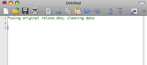
One optional step that can be helpful in creating do-files is placing a comment at the top of the file denoting which data you’re using and any other notes you want. To separate notes and comments from commands in do-files, begin the line with an asterisk. If it is a longer note, you can set it apart by typing /* before your comment and */ after the comment. For example, if I were using a data set called “relate”, I might begin my data file like this:

The first command you will need is the use command to specify the file you want Stata to use. If the file is not in the working directory that you are currently in, just specify which directory you want to pull the file from. Here are three examples of the use command, one from a data set in the current working directly, one from the internet and one from a jump drive in a different working directory. Notice that on the end of each command, I add the option clear. This is to clear any data that Stata is currently working with.

use relate.dta, clear
use http://www.stata-press.com/data/agis3/relate, clear
use "E:\relate.dta", clear

After I specify the data file, I enter the rest of the commands I want to run. Within this file, Stata will assume that each line is a new command unless you tell it otherwise. If you have a long command that you need on separate lines, add /// at the end of each line. That tells Stata that the next line is part of the same command. When I am ready to run the analyses, I select the commands I would like to run (you don’t have to select any text if you want to run them all) and click on the last icon on the toolbar in the do-file window:

To save your do-file, you can either use the icon on the toolbar or use the “File”->“Save As” menu while the do-file editor is active.

Creating log files

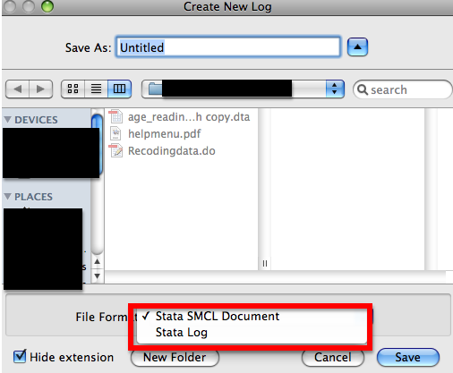
In addition to recording all of your commands in a do-file, you can also have Stata create a copy of everything that is sent to the Results window, with the exception of graphs. This is called a log file and can be helpful for you to save all of your output. This will also retain your commands, although it will not save them in the same way a do-file does (they will be embedded in the output). To create a log file, go to “File” -> “Log” -> “Begin.” This will bring up a dialogue box where you will save your log file. The default in Stata is to save the file with the extension .smcl. This will allow you to open the log file in Stata, but other programs will not read this type of file. The other extension available is .log. This file format will allow you to open your log file in other programs and may be easier to manage than the .smcl files. To save it as a .log file, just select the Stata Log option under the “File Format” menu in the dialogue box.

Once you begin a log file, you can suspend it at any time and resume later. You can do this by going to the “File” -> “Log” -> “Suspend” (or “Resume”). You can also close your log using this menu.

You can also start, suspend, resume and close logs using the log command. I will use this command to begin a log file, specify the name and location of the file as well as the extension. If I were going to create a log file called “creatinglogfiles” in a file on my desktop called “501” (filepath: /Desktop/501), I would type:

log using "/Desktop/501/creatinglogfiles", text

I included text because I want the file to be a .log file, not an .smcl file. If I wanted to overwrite a file that already existed, I would add replace after text.

After the log file is open, typing log off will suspend the log file, log on will resume the log file and log close will close your log file.

Stata: Reshaping Data

Reshaping Data

Reshaping

You will often have to reshape your data or change the name or values of your data to analyze it more easily. First, we’ll show you how to transform your data between “long” format, where there are multiple lines of data for every person, and “wide” format, where each subject has only one row and all data is entered in columns.

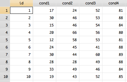
Right now, my data is in the “wide” format, where each participant reported their mood in four conditions.

However, for many analyses where participants have repeated measures, you will need your data in “long” format. In order to do this, you will use the reshape command, specifying that you’re reshaping to the long format. The syntax is reshape long/wide stubname, i(i) j(j) where the stubname is the stub of your variables (in this case, it is “cond”), i is the id variable and j is the new variable you’ll create (or the existing variable if reshaping the data into wide format).

reshape long cond, i(id) j(condition)

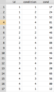
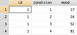
Now my data looks like this:

Now each participant has 4 rows with their reported mood in each condition. This may be confusing because “cond” actually reflects the value for mood in this data. So, in order to make your data more clear, you can use the rename command.

rename cond mood

Stata: Using generate to create new variables

Generating New Variables

The primary method for creating new variables in Stata is the generate command. Load the auto dataset.

clear
sysuse auto
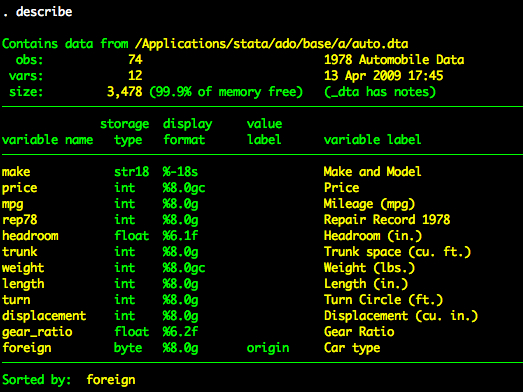
describe

New Variable from Existing Variables

Let’s create a new variable that is the sum of weight and length (ignore for the moment that summing weights and lengths doesn’t make a ton of sense). Simple with generate. The syntax of generate is:

generate nameOfNewVariable=whateverTheNewVariableIsEqualTo

So to create a new variable called weightlength that is the sum of weight and length we type:

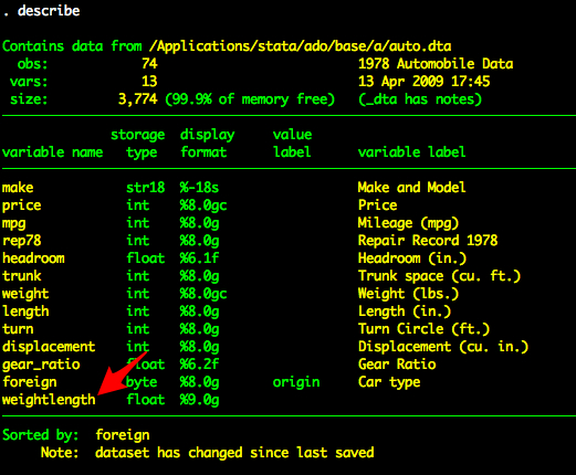
generate weightlength = weight+length

Now we have new variable called weightlength.

Suppose now that we want to create a new variable that is the square of weight.

generate weight2 = weight^2

New Variable that is a Constant

Suppose we want to create a new variable that is a constant value (this isn’t necessarily a good idea and you can use macros to store constants but using a variable can be pretty convenient too). Let’s make a new variable x that is equal to 100.

generate x = 100

Let’s create a new variable that is equal to the mean of weight – we’ll call it meanweight.

summarize weight

generate meanweight = 3019.459

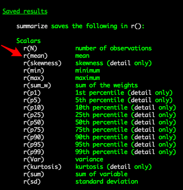
You can also use the results of the summarize command to create a mean.

summarize weight
generate meanweight = r(mean)

You can use the _N operator to create a new variable that is equal to the number of observations in a dataset.

generate obs = _N

If you combine this with by you can create a new variable that will be equal to the number of observations within the levels of the by variable. For example, we can type:

by foreign: generate obs = _N

This will create a variable that is a constant within the levels of foreign. That is, we are going to get the number of foreign cars and the number of domestic cars. If a line in the data is associated with foreign cars the new obs variable will have a value of 22 and domestic cars will have a value of 52. Give it a try and see how it works.

New Variable that is a Random Draw from a Distribution

We can create a new variable that is a random draw from a distribution. Let’s create a new variable whose values will be random draws from a normal distribution with a mean of 0 and a standard deviation of 1. The random normal generator command is rnormal() (it defaults to a mean of 0 and standard deviation of 1 and it will draw as many values as there are observations in the dataset).

generate random = rnormal()

Create a New Variable that Indexes the Observations

You can use the _n operator to create a variable that indexes the observation number.

generate index = _n

This will create a new variable that runs from 1 to 74. You can combine this with by to create an index within another variable.

by foreign: index = _n

This will create a new variable that runs from 1 to 52 for domestic cars and 1 to 22 for foreign cars.

Conclusion

I’ve just touched on the ways you can create new variables. You can also use the egen command to create new variables. Try new ways to create variables and be sure to read the help files.