Stata: Planned Comparisons with the test command

Planned Comparisons

This post will show you how to:

1. Run a one-way ANOVA using an independent variable with four levels.
2. Use planned comparisons to contrast levels of the independent variable.

We will use the built-in dataset systolic.

webuse systolic

Examining the data

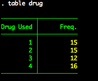
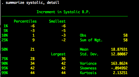
We will treat the systolic variable as the outcome and drug as the independent variable. Let’s look at descriptive statistics for systolic and frequencies for drug.

summarize systolic, detail

table drug

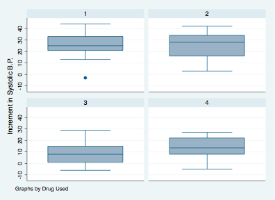
Let’s also look at a boxplot of systolic by drug.

graph box systolic, by(drug)

Thus, it appears there are some differences between drug levels and systolic blood pressure.

Oneway ANOVA

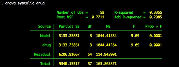
Let’s run a oneway ANOVA. The null hypothesis is that there is no difference in the mean systolic blood pressure among the levels of drug.

anova systolic drug

We reject the null hypothesis.

Using the test command to perform planned comparisons

In Stata, once we have completed the ANOVA, we can use the test command to perform planned comparisons. Note two important things about the test command:

1. You can only use it after you have run the ANOVA. If you try to run it before you run the ANOVA, it won’t work.
2. The test command is available to use for the most recently run model. If you run a second (or third, fourth, etc.) ANOVA model or another model that supports the test command (e.g., a regression) after you run the ANOVA you care about, you won’t be able to run the analysis you care about. That is, the information that test needs will not be available if you run another model.

Let’s say we want to know whether the average of drugs 1 and 2 differ from the averages of 3 and 4. To do this, we’d type the following command (after we ran the ANOVA).

test (1.drug + 2.drug)/2 = (3.drug + 4.drug)/2

We reject the null hypothesis that they are not different. Note that to reference levels of the variable drug we type 1.drug or 2.drug, etc. We put the level number, then a period, then the variabl ename. See if you can figure out why the following statement is equivalent

test (1.drug + 2.drug)/2 - (3.drug + 4.drug)/2 = 0

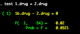
Suppose we want to know if level 1 of drug is different from level 2.

test 1.drug = 2.drug

We cannot reject reject the null.

The test command is really quite flexible. Fiddle around with it to better learn the syntax.

Stata: Oneway ANOVA

Oneway ANOVA

This post will show how to use the anova and loneway commands in Stata to compute a oneway ANOVA. We will use the auto dataset for this illustration. We will use price as the outcome variable and foreign as the factor.

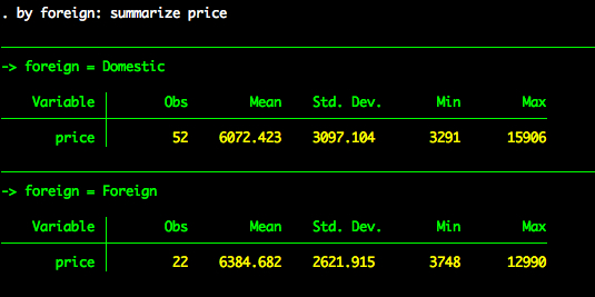
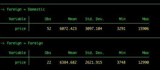
Let’s initially look at descriptive statistics for price stratified by foreign.

So it looks like there is a difference between in price between foreign and domestic cars, with foreign cars costing more money. We can test whether this difference is statistically significant with a oneway ANOVA (you could also just a use a t-test since there are just two levels of foreign).

anova Command

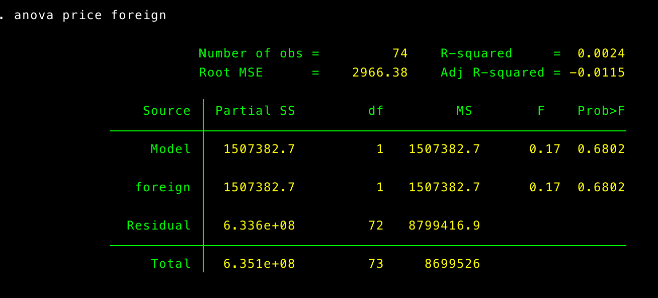
The anova command is simple and follows the standard Stata syntax – Command DV IV

anova price foreign

Viola – you’ve got an ANOVA source table.

Looks like the difference in price is not statistically significant. The advantage of using anova is that you can fit lots of different ANOVA models using this command (e.g., factorial ANOVA, repeated measures ANOVA, nested ANOVA). However, if you just want to fit a oneway ANOVA, then you can use the loneway command.

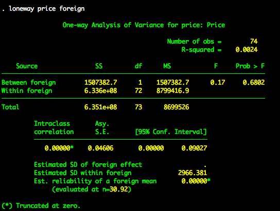
loneway Command

The loneway command is just for oneway ANOVA models. It provides output in addition to the source table, such as the intraclass correlation and the reliability of the group means. So depending upon the analysis you want to do and the information you need, loneway can be really useful.

loneway price foreign

Stata: Descriptive Statistics - Mean, median, variability

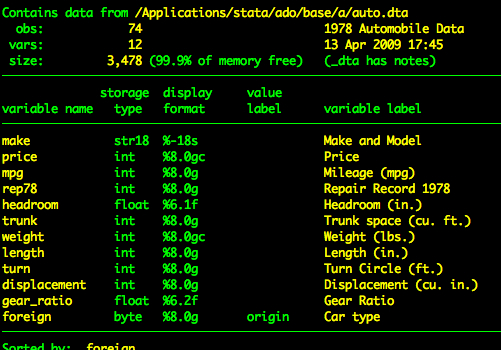
##Descriptive Statistics## For this tutorial we are going to use the auto dataset that comes with Stata. To load this data type

sysuse auto, clear

The auto dataset has the following variables.

describe

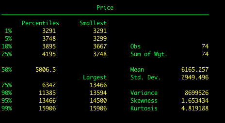
Suppose we want to get some summarize statistics for price such as the mean, standard deviation, and range. We’ll use the summarize command.

summarize price

Now let’s add the option detail to summarize. This will give us lots more information, including the median and other percentiles.

summarize price, detail

##Multiple Variables at Once##

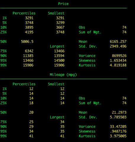
To get descriptives for multiple variables at once just add the variable names after summarize.

summarize price mpg

Adding the detail option.

summarize price mpg, detail

##Using by processing##

Suppose we want to get the descriptive statistics for price by car type (foreign vs domestic). We can use what is called by processing.

by foreign: summarize price

When using the by command, the variable of interest needs to be sorted in the data set. For example, in the previous example the variable “foreign” is already sorted within our data set. If we wanted to examine the price by mpg, we would need to sort miles per gallon. One way to sort data is using a simple sort command followed by the variable name. Stata will sort the data in ascending order by default.

sort mpg

After we sort the data, we can then use the standard by mpg: command. In by processing, we can also sort the data and execute the by command at the same time using the bysort command:

bysort mpg: summarize price

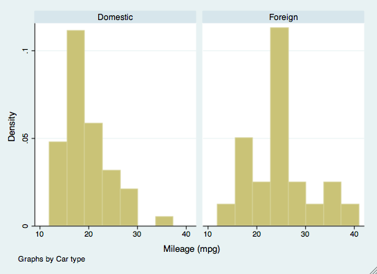
The by command can also be used in other commands, such as creating graphics. For example, if we wanted to examine histograms of mpg by the make of the car, we would use the by command as an option. The make of car does not have to be sorted for this command.

histogram(mpg), by(foreign)

##Using if##

The by statement will give us descriptives for all levels of the by variable (i.e., both foreign and domestic). Suppose we just want the describes for one level of the by variable. We can use the if statement for that. For foreign cars (i.e., foreign == 1):

summarize price if foreign == 1

For domestic cars (i.e., foreign == 0)

summarize price if foreign == 0

This table is to help in determining how to specify what levels of the variable you want to use.

Using in

The in qualifier specifies a particular subset of cases based on their order in the dataset. For example, if we want to examine the mpg in the 10 least expensive cars, we would use the in command.

sort price
summarize mpg in 1/10

As a helpful hint for any of these processes, if your variables are labeled (showing the label instead of the numeric value) and you need to find the numeric values to examine levels of the variable, you can use the nolabel option.

browse, nolabel

This will show you the number values for variables. You can also find those values by double-clicking on them in the data browser.

Things I Love About Stata -- egen mean

egen mean

I work a lot with clustered data, including group psychotherapy data (people clustered in groups), individual psychotherapy data (people clustered within therapists), and longitudinal data (observations clustered within people). Consequently, I often need to create cluster-level means and grand means for graphing and modeling. The egen mean function makes creating means easy. Combining egen mean with by processing in Stata makes this a breeze, even when cluster sizes differ.

egen mean for grand means

The egen function is used to create new variables. To create a mean with egen we use the following syntax:

egen nameofnewvariable=mean(nameofoldvariable)

We can download the the pig data from the xtmixed help.

webuse pig, clear

The variables are id, week, and weight.

list in 1/15, clean
id week weight
1. 1 1 24
2. 1 2 32
3. 1 3 39
4. 1 4 42.5
5. 1 5 48
6. 1 6 54.5
7. 1 7 61
8. 1 8 65
9. 1 9 72
10. 2 1 22.5
11. 2 2 30.5
12. 2 3 40.5
13. 2 4 45
14. 2 5 51
15. 2 6 58.5

We can create a grand mean (say, for creating centered variables) of weight using egen.

egen grandweight=mean(weight)

This creates a new variable that is equal to the grand mean for weight (it is a constant across all variables)

list in 1/15, clean
id week weight grandw~t
1. 1 1 24 50.40509
2. 1 2 32 50.40509
3. 1 3 39 50.40509
4. 1 4 42.5 50.40509
5. 1 5 48 50.40509
6. 1 6 54.5 50.40509
7. 1 7 61 50.40509
8. 1 8 65 50.40509
9. 1 9 72 50.40509
10. 2 1 22.5 50.40509
11. 2 2 30.5 50.40509
12. 2 3 40.5 50.40509
13. 2 4 45 50.40509
14. 2 5 51 50.40509
15. 2 6 58.5 50.40509

##egen mean for cluster means##

We can combine egen mean with by to compute cluster means. (Remember that id is the cluster id variable.)

by id: egen groupweight=mean(weight)

If the id variable isn’t sorted, then you can change the code to:

by id, sort: egen groupweight=mean(weight)

This creates a variable that is equal to the cluster mean for each cluster. That is, its value is constant within clusters but varies across clusters.

list in 1/15, clean
id week weight grandw~t groupw~t
1. 1 1 24 50.40509 48.66667
2. 1 2 32 50.40509 48.66667
3. 1 3 39 50.40509 48.66667
4. 1 4 42.5 50.40509 48.66667
5. 1 5 48 50.40509 48.66667
6. 1 6 54.5 50.40509 48.66667
7. 1 7 61 50.40509 48.66667
8. 1 8 65 50.40509 48.66667
9. 1 9 72 50.40509 48.66667
10. 2 1 22.5 50.40509 51.33333
11. 2 2 30.5 50.40509 51.33333
12. 2 3 40.5 50.40509 51.33333
13. 2 4 45 50.40509 51.33333
14. 2 5 51 50.40509 51.33333
15. 2 6 58.5 50.40509 51.33333

##Looking at missing data##

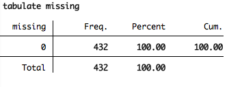
You can also use egen to generate a variable to examine missing data on each row. This can be particularly important when you are generating scale variables, or variables that will be combining values of multiple variables. For example, in the pig data above, if they were to weigh the pigs a second time (weight2) and create a variable of the difference between Time 1 and 2, if any pig were missing one of the time points, the difference score would not be accurate. In this hypothetical example, you could use egen combined with rowmiss to create a missing variable to examine this:

egen missing = rowmiss(weight weight2)

Then you can use the tabulate command to identify if any values are missing:

tabulate missing

Take a look at the other functions of egen–they’re remarkably useful.

Stata: Reading in Comma Separated Files

#Reading in Comma Separated Files#

This post will show how to read in comma separated files (also known as .csv files) into Stata. I will show you how to use both syntax and point-and-click.

##Syntax## You can import csv files using the insheet command.

insheet using "auto.csv", comma clear

The using auto.csv statement just tells Stata the file name of the csv file. If the csv file is not in your working directory, then you will need to provide the entire filepath or cd to the directory with the csv file. I typically include the option comma. This tells Stata that the file is a csv file. This isn’t necessary but it will speed up the insheet command (only an issue if the csv file is pretty big). However, the primary reason I put it in there is to make the code more readable (i.e., so that I know from the code that I read in a csv file, which is particularly important if the file extension is something other than csv). I also add the clear option to clear out any data that are currently in memory.

##Point-and-Click##

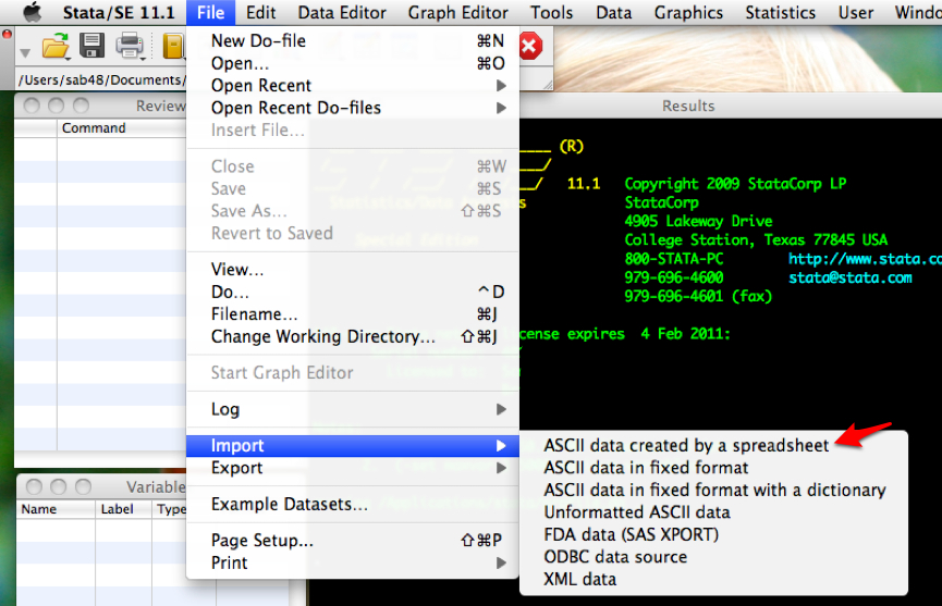
We can import csv files by using the Import submenu under the File menu. We’ll select ASCII data created by a spreadsheet under the Import submenu.

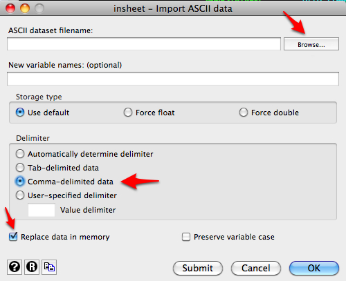
This will open the following dialog menu.

Click on Browse to select the csv file saved on your computer. Select Comma-delimited data. I’ve also selected Replace data in memory to clear out any data loaded into Stata already. If you need to add variable names, you can add them in the dialog box.

Now your data will be read into Stata and ready to use.